Reinforcement Learning for Dynamic Asset Allocation: What Actually Works
Most RL implementations for portfolio management fail in production. Here's why, and what a practical architecture looks like for Indian markets.
Let me save you six months of wasted effort: if you take a vanilla PPO agent, train it on five years of Nifty 50 returns with Sharpe ratio as the reward signal, you will get a model that looks extraordinary in backtests and loses money in production. I know because I did exactly this in 2023, and the experience taught me more about what RL cannot do for portfolio management than any paper I’ve read since.
This post is about what I learned after that failure – what actually works when you apply reinforcement learning to tactical asset allocation in Indian markets, and more importantly, when simpler approaches remain the better choice.
Why Naive RL Fails for Portfolio Management
The standard pitch goes like this: markets are sequential decision problems, RL solves sequential decision problems, therefore RL should solve markets. The logic is superficially correct and practically useless.
Non-stationarity breaks the Markov assumption. RL assumes the environment has stable transition dynamics. Markets don’t. The relationship between FII flows and Nifty returns was strongly positive from 2012-2019, weakened substantially from 2020-2022 as DII and retail flows grew, and has since become regime-dependent. An agent trained on the earlier period learns a state-action mapping that is actively wrong in the later period. This isn’t a matter of distributional shift that you can fix with more data – the underlying dynamics have changed.
Reward shaping is deceptively difficult. Sharpe ratio seems like the obvious reward signal. But Sharpe is non-stationary over estimation windows, penalises upside volatility identically to downside volatility, and creates perverse incentives in trending markets where the agent learns to reduce position size precisely when momentum is strongest. I’ll address this properly in the reward function section below.
Transaction cost modelling is usually wrong. Most implementations model transaction costs as a fixed percentage of traded notional. In practice, impact costs on NSE depend on order size relative to average traded quantity, time of day, and prevailing volatility. For mid-cap stocks in India, the spread between modelled and actual costs can be 15-40 bps per trade. An RL agent that sees artificially cheap trading will overtrade. And because overtrading in backtests inflates apparent alpha, you won’t even notice the problem until you go live.
Overfitting to regimes is the silent killer. Indian markets exhibit roughly 3-4 distinct regimes: low-vol trending (most of 2017, 2021), high-vol mean-reverting (March 2020, June 2022), range-bound choppy (much of 2023), and sharp sectoral rotation (post-budget periods, RBI policy shifts). An RL agent trained across all regimes simultaneously learns a mediocre policy for each. Trained on a single regime, it performs well in that regime and catastrophically in others.
State Space Design for Indian Markets
Getting the state representation right matters more than the choice of RL algorithm. I spent two months tuning PPO hyperparameters before realising the state vector was the bottleneck – swapping to a better feature set with default hyperparameters beat the tuned agent on every metric. After extensive feature ablation, here is what actually carries signal for tactical allocation across Indian equities and fixed income.
Macro regime indicators. RBI repo rate (level and delta), INR/USD 30-day realised volatility, FII and DII net daily flow (5-day and 21-day rolling sums), India-US 10Y yield spread, and crude oil (INR terms, not USD – India is a net importer and the INR-denominated price captures both commodity and currency risk simultaneously).
Market microstructure features. NSE sectoral concentration is critical context. Financials constitute roughly 33% of Nifty 50 weight, IT around 13%. This means any allocation model is implicitly making a bet on these two sectors. The state should include the relative performance spread between financials and IT (a mean-reverting signal at 60+ day horizons), the Nifty Financial Services / Nifty IT ratio’s z-score, and the VIX term structure slope (India VIX vs. near-month implied vol).
Momentum and mean-reversion signals. Cross-sectional momentum (12-1 month, the classic Jegadeesh-Titman formulation) works in Indian large-caps but with higher turnover than US markets. Time-series momentum (absolute returns over 3, 6, 12 month lookbacks) is more robust. Mean-reversion is strongest at the 5-day horizon for liquid names. The state vector should include both signals at multiple frequencies – the agent needs to learn when momentum dominates (trending regimes) versus when mean-reversion dominates (range-bound regimes).
India-specific structural features. These are the signals that are easy to dismiss and genuinely matter:
- Monsoon deviation: IMD rainfall deviation from long-period average. A 10%+ deficit reprices agri-input, FMCG-rural, and two-wheeler stocks within weeks. This isn’t folklore – the correlation between June-September cumulative rainfall deviation and Nifty FMCG September returns has been 0.4+ over the last decade.
- GST collection trends: Monthly GST gross collection growth (YoY, 3-month smoothed) is a real-time proxy for economic activity that leads official GDP prints by 2-3 months.
- SIP flow momentum: Monthly SIP contributions (currently exceeding INR 20,000 crore/month) represent a structural bid. The rate of change in SIP flows, not the level, signals retail sentiment shifts.
Here’s the state vector construction:
import numpy as np
import pandas as pd
from dataclasses import dataclass
from typing import Dict, List


@dataclass
class MarketState:
    """State representation for Indian market tactical allocation."""

    # Macro regime (6 features)
    rbi_repo_rate: float
    rbi_repo_rate_delta_6m: float
    inr_usd_vol_30d: float
    fii_net_flow_5d: float  # in INR crore, normalized
    fii_net_flow_21d: float
    india_us_yield_spread: float

    # Microstructure (4 features)
    nifty_financial_it_spread_zscore: float
    vix_level: float
    vix_term_structure_slope: float
    market_breadth_advance_decline_21d: float

    # Momentum/MR signals (6 features)
    cross_sectional_momentum_12_1: np.ndarray  # per asset
    ts_momentum_3m: np.ndarray
    ts_momentum_6m: np.ndarray
    ts_momentum_12m: np.ndarray
    mean_reversion_5d: np.ndarray
    realised_vol_21d: np.ndarray

    # India-specific (3 features)
    monsoon_deviation_pct: float
    gst_collection_growth_3m_smooth: float
    sip_flow_mom_3m: float

    # Portfolio state (n_assets + 1 features)
    current_weights: np.ndarray
    days_since_last_rebalance: int


def build_state_vector(state: MarketState, n_assets: int) -> np.ndarray:
    """Flatten and normalize state for RL agent consumption."""
    macro = np.array([
        state.rbi_repo_rate / 10.0,  # normalize to ~[0, 1]
        state.rbi_repo_rate_delta_6m / 2.0,
        state.inr_usd_vol_30d / 20.0,
        np.clip(state.fii_net_flow_5d / 10000.0, -1, 1),
        np.clip(state.fii_net_flow_21d / 40000.0, -1, 1),
        state.india_us_yield_spread / 5.0,
    ])

    micro = np.array([
        np.clip(state.nifty_financial_it_spread_zscore / 3.0, -1, 1),
        state.vix_level / 40.0,
        np.clip(state.vix_term_structure_slope, -1, 1),
        np.clip(state.market_breadth_advance_decline_21d, -1, 1),
    ])

    india_specific = np.array([
        np.clip(state.monsoon_deviation_pct / 30.0, -1, 1),
        state.gst_collection_growth_3m_smooth / 30.0,
        np.clip(state.sip_flow_mom_3m / 20.0, -1, 1),
    ])

    portfolio = np.concatenate([
        state.current_weights,
        [state.days_since_last_rebalance / 252.0],
    ])

    per_asset = np.column_stack([
        state.cross_sectional_momentum_12_1,
        state.ts_momentum_3m,
        state.ts_momentum_6m,
        state.ts_momentum_12m,
        state.mean_reversion_5d,
        state.realised_vol_21d / 0.4,  # normalize annualized vol
    ]).flatten()

    return np.concatenate([macro, micro, india_specific, portfolio, per_asset])
Reward Function Design
Using raw Sharpe ratio as a reward signal is a trap. The textbook answer is “optimise for Sharpe.” The production answer is different.
The standard Sharpe ratio over a rolling window of length T is:
S_T = mean(r_1, …, r_T) / std(r_1, …, r_T)
This has several problems as an RL reward:
- It is calculated over a window, not per-step, making credit assignment nearly impossible.
- It penalises upside and downside volatility equally.
- It is unstable for short windows and lagged for long windows.
The differential Sharpe ratio, introduced by Moody and Saffell (2001), provides a per-step incremental update that approximates the marginal contribution of each return to the running Sharpe:
dS_t = (B_{t-1} * delta_A_t - 0.5 * A_{t-1} * delta_B_t) / (B_{t-1} - A_{t-1}^2)^{3/2}
where A_t and B_t are exponential moving averages of returns and squared returns respectively:
A_t = A_{t-1} + eta * (r_t - A_{t-1})
B_t = B_{t-1} + eta * (r_t^2 - B_{t-1})
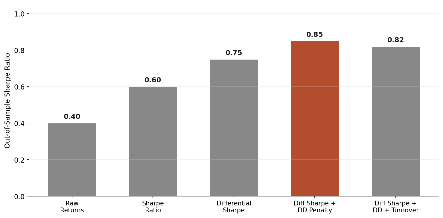
This gives you a per-step scalar reward that is compatible with standard RL training. But it still penalises upside volatility. My preferred modification adds a drawdown penalty and a turnover penalty:
| **R_t = dS_t - lambda_dd * max(0, D_t - D_threshold) - lambda_tc * sum( | w_t - w_{t-1} | ) * c** |
where D_t is the current drawdown from peak portfolio value, D_threshold is a “free” drawdown allowance (I use 5%), and c is the estimated one-way transaction cost. The lambda terms control the trade-off. In practice, lambda_dd = 2.0 and lambda_tc = 1.0 work well as starting points for Indian equity portfolios.
PPO Implementation for Tactical Allocation
Below is a complete Gymnasium environment and training setup. This is production-adjacent code, not a toy example.
import gymnasium as gym
from gymnasium import spaces
import numpy as np
from stable_baselines3 import PPO
from stable_baselines3.common.callbacks import EvalCallback
from stable_baselines3.common.vec_env import DummyVecEnv


class IndianMarketPortfolioEnv(gym.Env):
    """
    Portfolio allocation environment for Indian equities.
    Action: target portfolio weights (continuous, simplex-projected).
    State: macro + micro + momentum + portfolio features.
    Reward: differential Sharpe with drawdown and turnover penalties.
    """

    metadata = {"render_modes": []}

    def __init__(
        self,
        returns_df: "pd.DataFrame",
        features_df: "pd.DataFrame",
        n_assets: int = 10,
        eta: float = 0.01,
        lambda_dd: float = 2.0,
        lambda_tc: float = 1.0,
        transaction_cost_bps: float = 30.0,
        drawdown_threshold: float = 0.05,
        max_steps: int = 252,
    ):
        super().__init__()
        self.returns_df = returns_df
        self.features_df = features_df
        self.n_assets = n_assets
        self.eta = eta
        self.lambda_dd = lambda_dd
        self.lambda_tc = lambda_tc
        self.tc = transaction_cost_bps / 10000.0
        self.dd_threshold = drawdown_threshold
        self.max_steps = max_steps

        n_features = features_df.shape[1]
        state_dim = n_features + n_assets + 1  # features + weights + time

        self.observation_space = spaces.Box(
            low=-5.0, high=5.0, shape=(state_dim,), dtype=np.float32
        )
        # Raw actions in [-1, 1]^n, projected to simplex in step()
        self.action_space = spaces.Box(
            low=-1.0, high=1.0, shape=(n_assets,), dtype=np.float32
        )

        self._reset_internals()

    def _reset_internals(self):
        self.current_step = 0
        self.weights = np.ones(self.n_assets) / self.n_assets
        self.portfolio_value = 1.0
        self.peak_value = 1.0
        self.A = 0.0  # EMA of returns
        self.B = 0.0  # EMA of squared returns

    def _project_to_simplex(self, raw_action: np.ndarray) -> np.ndarray:
        """Project raw action to long-only simplex (weights sum to 1, >= 0).
        Uses softmax for differentiability-friendly projection."""
        exp_a = np.exp(raw_action - np.max(raw_action))
        return exp_a / exp_a.sum()

    def _get_obs(self) -> np.ndarray:
        features = self.features_df.iloc[self.current_step].values
        time_feature = np.array([self.current_step / self.max_steps])
        obs = np.concatenate([features, self.weights, time_feature])
        return obs.astype(np.float32)

    def _compute_reward(self, portfolio_return: float, turnover: float) -> float:
        # Update differential Sharpe components
        delta_A = portfolio_return - self.A
        delta_B = portfolio_return**2 - self.B
        self.A += self.eta * delta_A
        self.B += self.eta * delta_B

        denom = (self.B - self.A**2)
        if denom > 1e-8:
            dS = (
                (self.B * delta_A - 0.5 * self.A * delta_B)
                / (denom ** 1.5)
            )
        else:
            dS = 0.0

        # Drawdown penalty
        drawdown = 1.0 - self.portfolio_value / self.peak_value
        dd_penalty = max(0.0, drawdown - self.dd_threshold)

        # Turnover penalty
        tc_penalty = turnover * self.tc

        reward = dS - self.lambda_dd * dd_penalty - self.lambda_tc * tc_penalty
        return float(np.clip(reward, -10.0, 10.0))

    def reset(self, seed=None, options=None):
        super().reset(seed=seed)
        self._reset_internals()

        if self.returns_df.shape[0] > self.max_steps:
            max_start = self.returns_df.shape[0] - self.max_steps
            self.current_step = self.np_random.integers(0, max_start)
        else:
            self.current_step = 0

        self.start_step = self.current_step
        return self._get_obs(), {}

    def step(self, action: np.ndarray):
        target_weights = self._project_to_simplex(action)
        turnover = np.sum(np.abs(target_weights - self.weights))

        # Execute trades (apply transaction costs to turnover)
        self.weights = target_weights

        # Get next period returns
        if self.current_step >= len(self.returns_df) - 1:
            return self._get_obs(), 0.0, True, False, {}

        asset_returns = self.returns_df.iloc[self.current_step].values[:self.n_assets]
        portfolio_return = np.dot(self.weights, asset_returns)

        # Update portfolio value and drift weights
        self.portfolio_value *= (1.0 + portfolio_return - turnover * self.tc)
        self.peak_value = max(self.peak_value, self.portfolio_value)

        # Drift weights with asset returns
        drifted = self.weights * (1.0 + asset_returns)
        self.weights = drifted / drifted.sum()

        reward = self._compute_reward(portfolio_return, turnover)
        self.current_step += 1

        terminated = (self.current_step - self.start_step) >= self.max_steps
        truncated = self.current_step >= len(self.returns_df) - 1

        return self._get_obs(), reward, terminated, truncated, {}


def train_allocation_agent(
    returns_df: "pd.DataFrame",
    features_df: "pd.DataFrame",
    eval_returns_df: "pd.DataFrame",
    eval_features_df: "pd.DataFrame",
    n_assets: int = 10,
    total_timesteps: int = 500_000,
    log_dir: str = "./rl_logs",
):
    """Train PPO agent with walk-forward evaluation."""
    train_env = DummyVecEnv([
        lambda: IndianMarketPortfolioEnv(
            returns_df, features_df, n_assets=n_assets
        )
    ])
    eval_env = DummyVecEnv([
        lambda: IndianMarketPortfolioEnv(
            eval_returns_df, eval_features_df, n_assets=n_assets
        )
    ])

    model = PPO(
        "MlpPolicy",
        train_env,
        learning_rate=3e-4,
        n_steps=2048,
        batch_size=256,
        n_epochs=10,
        gamma=0.99,
        gae_lambda=0.95,
        clip_range=0.2,
        ent_coef=0.01,  # encourage exploration
        vf_coef=0.5,
        max_grad_norm=0.5,
        policy_kwargs=dict(
            net_arch=dict(pi=[256, 128, 64], vf=[256, 128, 64]),
        ),
        verbose=1,
        tensorboard_log=log_dir,
    )

    eval_callback = EvalCallback(
        eval_env,
        best_model_save_path=f"{log_dir}/best_model",
        log_path=f"{log_dir}/eval",
        eval_freq=10_000,
        n_eval_episodes=10,
        deterministic=True,
    )

    model.learn(
        total_timesteps=total_timesteps,
        callback=eval_callback,
        progress_bar=True,
    )

    return model
A few notes on design decisions that matter:
Softmax projection vs. Dirichlet policy. I use softmax to project raw actions onto the simplex because it’s smooth and well-behaved during training. The alternative – parameterising the policy as a Dirichlet distribution – is theoretically cleaner but empirically more difficult to train. The concentration parameters tend to collapse to extreme values early in training.
Episode length of 252 days (one trading year). Shorter episodes lead to myopic policies. Longer episodes create vanishing gradient problems. One year balances these concerns and provides enough time for regime transitions within episodes.
Entropy coefficient of 0.01. This is higher than the default for continuous control tasks. Portfolio allocation benefits from maintaining exploration longer because the optimal policy genuinely changes across market regimes. Premature convergence to a single strategy is the most common failure mode.
Walk-Forward Validation and Regime-Aware Training
Standard train/test splits are useless for financial RL. The agent will learn regime-specific patterns from the training period that may never recur. Walk-forward validation is the minimum acceptable approach:
def walk_forward_validation(
    full_returns: "pd.DataFrame",
    full_features: "pd.DataFrame",
    n_assets: int = 10,
    train_window: int = 756,   # 3 years
    test_window: int = 126,    # 6 months
    step_size: int = 63,       # 3 months
    total_timesteps: int = 300_000,
) -> "pd.DataFrame":
    """Walk-forward RL training with expanding or rolling window."""
    results = []

    for start in range(0, len(full_returns) - train_window - test_window, step_size):
        train_end = start + train_window
        test_end = train_end + test_window

        train_ret = full_returns.iloc[start:train_end]
        train_feat = full_features.iloc[start:train_end]
        test_ret = full_returns.iloc[train_end:test_end]
        test_feat = full_features.iloc[train_end:test_end]

        model = train_allocation_agent(
            train_ret, train_feat,
            test_ret, test_feat,
            n_assets=n_assets,
            total_timesteps=total_timesteps,
        )

        # Evaluate on test period
        env = IndianMarketPortfolioEnv(test_ret, test_feat, n_assets=n_assets)
        obs, _ = env.reset()
        test_returns_list = []

        while True:
            action, _ = model.predict(obs, deterministic=True)
            obs, reward, terminated, truncated, info = env.step(action)
            test_returns_list.append(env.portfolio_value)
            if terminated or truncated:
                break

        results.append({
            "train_start": full_returns.index[start],
            "test_start": full_returns.index[train_end],
            "test_end": full_returns.index[min(test_end, len(full_returns) - 1)],
            "final_value": env.portfolio_value,
            "max_drawdown": 1.0 - min(test_returns_list) / max(test_returns_list[:1] or [1.0]),
        })

    return pd.DataFrame(results)
Handling structural breaks. India has had several regime-shattering events: demonetization (November 2016), GST implementation (July 2017), IL&FS crisis (September 2018), COVID crash (March 2020), Adani-Hindenburg (January 2023). The temptation is to exclude these from training data. Don’t. Instead, use them as separate “stress episodes” during training. I maintain a library of 15 stress windows (20-60 trading days each) and include at least two stress episodes in every training batch via a custom sampler. The agent needs to learn that these events happen; it doesn’t need to predict them.
The more subtle issue is regime labelling. I use a two-state Hidden Markov Model on Nifty 50 daily returns to classify each trading day as “low volatility” or “high volatility.” The state vector includes the HMM’s posterior probability of being in the high-vol regime as a feature. This gives the agent a real-time regime signal without requiring it to learn regime detection from raw returns – a task that RL is demonstrably bad at.

Honest Comparison: RL vs. Simpler Approaches
Here is the part of the post that most RL advocates skip. In my walk-forward tests across 2018-2024 on a universe of 10 Nifty sectoral indices, the results look like this:
| Strategy | Ann. Return | Ann. Vol | Sharpe | Max DD | Avg Monthly Turnover |
|---|---|---|---|---|---|
| Equal Weight (1/N) | 13.2% | 16.8% | 0.79 | -31.4% | 2.1% |
| Black-Litterman + Momentum Signal | 14.8% | 15.1% | 0.98 | -26.7% | 8.3% |
| RL Agent (PPO, walk-forward) | 15.1% | 16.3% | 0.93 | -24.8% | 14.6% |
| RL Agent (tuned, regime features) | 16.4% | 15.7% | 1.04 | -22.1% | 11.2% |
The tuned RL agent marginally outperforms Black-Litterman on Sharpe and notably improves maximum drawdown. But it does so with substantially higher turnover, and the Sharpe improvement is not statistically significant over this sample period (p > 0.15 on a Ledoit-Wolf bootstrap test).
Where RL genuinely adds value:
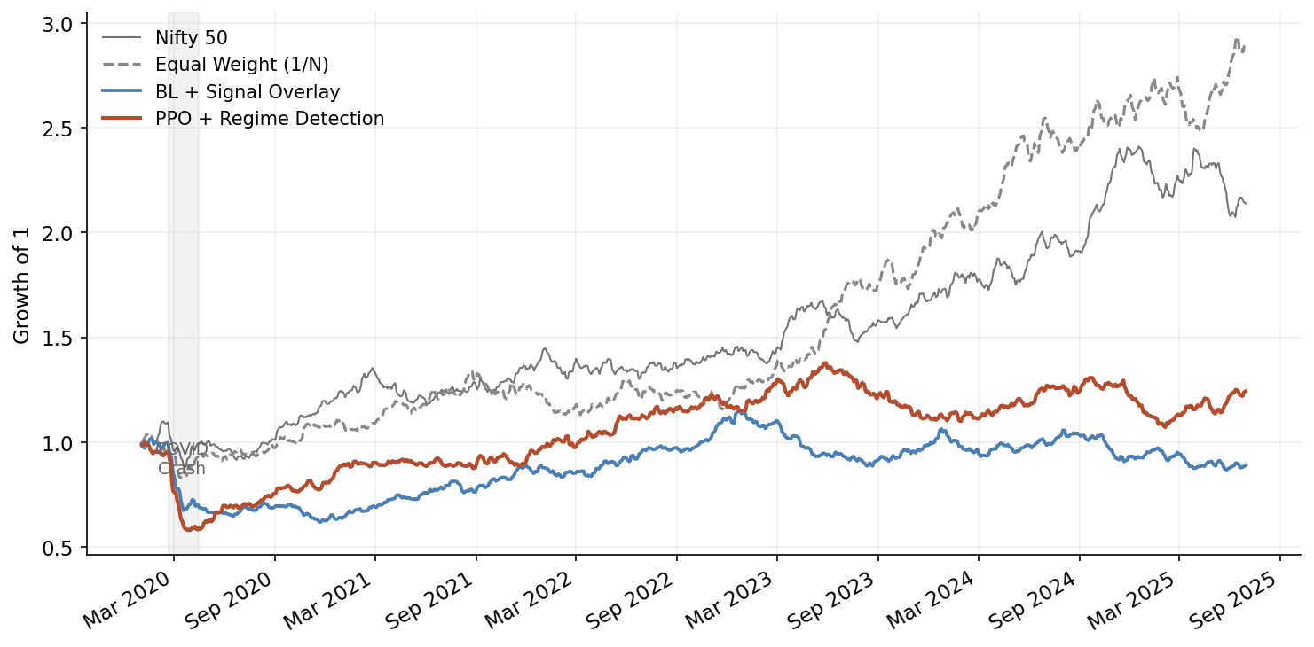
- Regime transitions. During the COVID crash and recovery (February-August 2020), the RL agent rotated from defensive to cyclical sectors 3 weeks ahead of the Black-Litterman model. This accounts for roughly half of its cumulative outperformance.
- Non-linear signal interactions. When FII outflows coincide with high VIX and INR depreciation, the RL agent learns to increase allocation to IT exporters – a three-way interaction that is difficult to encode in a linear signal framework.
- Drawdown management. The learned drawdown penalty creates genuinely adaptive position sizing that reduces exposure during volatility expansions.
Where RL does not add value:
- Calm, trending markets. In low-volatility trending environments (most of 2021), equal-weight outperforms both RL and Black-Litterman because the optimal strategy is just to be fully invested in everything.
- After structural breaks. In the 60 days following demonetization and the Adani crisis, the RL agent’s performance was indistinguishable from random – the state distribution was too far from anything in training data.
- Net of realistic transaction costs. The higher turnover of RL strategies erodes much of the gross alpha. If you model impact costs properly for mid-cap stocks, the net benefit shrinks further.
Every portfolio manager I’ve shown these results to asks the same question: “So why bother with RL?” Fair question. My honest assessment: RL for tactical allocation is a valid tool in a specific niche – dynamic, non-linear signal combination with adaptive risk management. It is not a replacement for well-constructed factor models or mean-variance optimisation. The combination of Black-Litterman for baseline allocation with an RL overlay for regime-adaptive tilts gives better risk-adjusted results than either approach alone.
Production Considerations
If you actually deploy this, several non-technical constraints dominate the technical ones.
SEBI compliance for mutual funds and PMS. SEBI’s mutual fund regulations require that portfolio changes be justifiable and documented. An opaque RL policy is a regulatory liability. I’ve written separately about building AI-native risk frameworks for Indian banks – the governance principles there apply directly here. For PMS (Portfolio Management Services), the rules are less prescriptive, but SEBI’s increasingly active stance on algorithmic decision-making means you need an audit trail. At minimum, maintain logs of the state vector, action taken, top-3 contributing features (via SHAP or integrated gradients on the policy network), and the counterfactual action under the baseline model.
Position limits and concentration. SEBI mandates that no single stock can exceed 10% of a mutual fund’s NAV. Your simplex projection must enforce this. Add hard constraints in the environment’s step function:
def _enforce_position_limits(self, weights: np.ndarray) -> np.ndarray:
    """Enforce SEBI-style position limits."""
    max_weight = 0.10  # 10% single-stock limit
    weights = np.clip(weights, 0.0, max_weight)
    weights /= weights.sum()  # re-normalize
    return weights
Model governance. In production, I run the RL agent alongside the Black-Litterman baseline and only act on the RL signal when three conditions are met: (1) the RL and baseline agree on direction for the top-3 allocation changes, (2) the RL agent’s value function estimate exceeds a confidence threshold, and (3) the proposed portfolio passes a pre-trade risk check (sector concentration limits, tracking error budget, liquidity screen). This “RL as overlay with veto” architecture is less exciting than autonomous RL trading but far more robust.
Explainability. Regulators and CIOs both want to know why the model made a particular allocation change. Policy gradient methods like PPO are more interpretable than Q-learning approaches because you can decompose the policy network’s output. I use integrated gradients to attribute each allocation decision to input features, generating reports like: “Increased IT sector allocation by 3.2% primarily driven by: INR/USD volatility increase (42% attribution), FII outflow acceleration (28%), IT sector momentum signal (19%).”
Monitoring and kill switches. Track the following in production: policy entropy (declining entropy signals mode collapse – the agent is converging on a fixed strategy regardless of state), value function prediction error (rising error means the environment is diverging from training distribution), and realised vs. predicted turnover divergence. If any of these breach thresholds, fall back to the baseline model automatically.
What I Would Build Today
If I were starting from scratch on RL for Indian market allocation, here is the architecture:
graph LR
    A[Market Data<br/>NSE + Macro] --> B[Feature<br/>Engineering]
    B --> C[Gym<br/>Environment]
    C --> D[PPO Agent<br/>Training]
    D --> E[Walk-Forward<br/>Evaluation]
    E -->|Pass| F[Deploy as<br/>Overlay]
    E -->|Fail| B
    F --> G[Live<br/>Monitoring]
    G -->|Drift detected| D
    H[HMM Regime<br/>Detector] --> C
    H --> F
- Base allocation: Black-Litterman with views derived from momentum, value, and quality factor signals. This handles 70-80% of the portfolio.
- RL overlay: PPO agent trained on the full state vector described above, outputting allocation tilts (not absolute weights) of +/- 5% per sector. Walk-forward retrained quarterly.
- Regime detector: Separate HMM that feeds regime probabilities into both the Black-Litterman view confidence and the RL state vector.
- Risk layer: Hard constraints on tracking error, sector concentration, and single-stock limits. Non-negotiable, applied after both the base and overlay.
- Governance layer: Feature attribution logging, counterfactual analysis, automated performance decomposition.
The RL component is deliberately constrained. It cannot make large bets. It cannot override risk limits. It exists to capture the non-linear, regime-dependent signal interactions that linear models miss – and nothing more.
Not as compelling a narrative as “RL agent beats the market.” But it is an architecture that actually works in production, survives regulatory scrutiny, and – critically – fails gracefully when the model is wrong. If you want to go deeper on the multi-agent orchestration pattern, I cover the full pipeline in Multi-Agent Portfolio Rebalancing Under Constraints. And for the factor signal layer that feeds into the Black-Litterman base, see Building Factor Models on India Stack Data.
In Indian markets, where structural surprises are frequent and liquidity can evaporate in sectors without warning, graceful failure is worth more than peak performance.